2. Using ImagePipelines to process batches

Learn to tune and use prefabricated image processing pipelines, then deploy them at scale.

---

In this tutorial, we’ll introduce how to use widgets to tune pipeline parameters, and process images at scale.

Note:

• We’ll also be using the same data in {doc}GrowthCurves.

import phenotypic as pht

filepaths = [x for x in
             pht.data.yield_sample_dataset(mode='filepath')]
# This returns the relative filepaths for this sample data
# While unconventional for a loader, this is done to demonstrate importing an directory of images.
filepaths

[PosixPath('../../../../../src/phenotypic/data/PhenoTypicSampleSubset/2_1S_5.jpg'),
 PosixPath('../../../../../src/phenotypic/data/PhenoTypicSampleSubset/2_1S_6.jpg'),
 PosixPath('../../../../../src/phenotypic/data/PhenoTypicSampleSubset/2_1S_7.jpg'),
 PosixPath('../../../../../src/phenotypic/data/PhenoTypicSampleSubset/2_1S_8.jpg'),
 PosixPath('../../../../../src/phenotypic/data/PhenoTypicSampleSubset/3_1S_5.jpg'),
 PosixPath('../../../../../src/phenotypic/data/PhenoTypicSampleSubset/3_1S_6.jpg'),
 PosixPath('../../../../../src/phenotypic/data/PhenoTypicSampleSubset/3_1S_7.jpg'),
 PosixPath('../../../../../src/phenotypic/data/PhenoTypicSampleSubset/3_1S_8.jpg'),
 PosixPath('../../../../../src/phenotypic/data/PhenoTypicSampleSubset/4_1S_5.jpg'),
 PosixPath('../../../../../src/phenotypic/data/PhenoTypicSampleSubset/4_1S_6.jpg'),
 PosixPath('../../../../../src/phenotypic/data/PhenoTypicSampleSubset/4_1S_7.jpg'),
 PosixPath('../../../../../src/phenotypic/data/PhenoTypicSampleSubset/4_1S_8.jpg'),
 PosixPath('../../../../../src/phenotypic/data/PhenoTypicSampleSubset/5_1S_5.jpg'),
 PosixPath('../../../../../src/phenotypic/data/PhenoTypicSampleSubset/5_1S_6.jpg'),
 PosixPath('../../../../../src/phenotypic/data/PhenoTypicSampleSubset/5_1S_7.jpg'),
 PosixPath('../../../../../src/phenotypic/data/PhenoTypicSampleSubset/5_1S_8.jpg'),
 PosixPath('../../../../../src/phenotypic/data/PhenoTypicSampleSubset/6_1S_5.jpg'),
 PosixPath('../../../../../src/phenotypic/data/PhenoTypicSampleSubset/6_1S_6.jpg'),
 PosixPath('../../../../../src/phenotypic/data/PhenoTypicSampleSubset/6_1S_7.jpg'),
 PosixPath('../../../../../src/phenotypic/data/PhenoTypicSampleSubset/6_1S_8.jpg')]

Processing your first image

---

Here we’re gonna import the last image in the dataset, since its from the last timepoint and should have reasonable growth. Accepted file formats are jpegs, tiffs, pngs, and RAW files.

Important things to note:

• bit_depth will have an important role in memory usage and accuracy. For jpegs, this will always be 8. For other image formats, consult your camera documentation for information. You may also find this information in your image metadata, depending on the format. PhenoTypic supports bit depths of 8 and 16. If not provided, PhenoTypic will try to guess this information from the imported image data.

# We're gonna import the last image in the dataset, lets make an image with a grid in 96 array format
# Accepted filepaths are jpegs, tiffs, pngs, and RAW format files
# These images are jpegs so we set a bit depth of 8.
image = pht.GridImage.imread(filepaths[-2], nrows=8, ncols=12, bit_depth=8)

Let’s then view the image. PhenoTypic uses matplotlib as the backend for compatibility, which allows for streamlined prototyping in Jupyter. All plotting methods return (plt.Figure, plt.Axes) for easy post-plotting editing. You can also plot directly to an axes. There’s a few different ways to view your image and its internal states.

1. View the input image

Image.show() # Shows the input image
fig, ax = Image.show() # If you need the figure or axes for further processing
fig.show()

2. Viewing specific components

rgb_fig, rgb_ax = Image.rgb.show() # Shows the rgb array if its available
gray_fig, gray_ax = Image.gray.show() # Shows the grayscale array.

Also available for other image components such as enh_gray, objmask, objmap, …

3. Viewing overlay information

overlay_fig, overlay_ax = Image.show_overlay()
overlay_fig.show()

fig, ax = image.show()

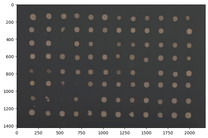
You can always visualize your image with Image.show(). This returns a matplotlib figure and axes object, but should plot the figures inside a jupyter notebook. The axis labels are the pixel rows and columns that show the size of your photo. If your original input is rgb or grayscale, Image.show() will return the original image. To show the grayscale converted version of your image, use Image.gray.show().

HeavyGitterPipeline

For ease of use, PhenoTypic supplies built-in pipelines that we have curated for different projects we use internally. Here’s a demo of the HeavyGitterPipeline.

The HeavyWatershedPipeline consists of the following operations:

1. BM3DDenoise

2. CLAHE

3. MedianFilter

4. GitterDetector

5. MaskOpener

6. BorderObjectRemover

7. SmallObjectRemover

8. MaskFill

9. GridOversizedObjectRemover

10. MinResidualRemover

11. GridAligner

12. GitterDetector (second pass since alignment might improve detection)

13. MaskOpener

14. BorderObjectRemover

15. SmallObjectRemover

16. MaskFill

17. MinResidualReducer

It also has the following measurements:

• MeasureShape

• MeasureIntensity

• MeasureTexture

• MeasureColor

You can apply ImagePipeline and ImageOperation in place or make a new copy for comparison.

# return a copy
new_image = pipe.apply(image)

# in place
pipe.apply(image, inplace=True)

from phenotypic.prefab import HeavyRoundPeaksPipeline

pipe = HeavyRoundPeaksPipeline()

To tune the parameters you can use the widget method that comes with every ImageOperation and ImagePipeline. This lets you visually interact with the parameters of the class. Pressing the Update View button will update the parameters and let you preview their effects on the image supplied as an argument to the method.

pipe.widget(image)

📝 Note: Interactive widgets in documentation

When viewing this tutorial as static HTML documentation, widgets will appear as images. For full interactivity, run this notebook in Jupyter Notebook or JupyterLab.

pipe.apply(image, inplace=True)

fig, ax = image.show_overlay()  # returns a figure and axes

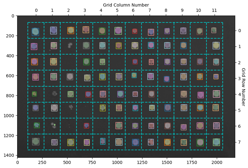
Here the objects with a colored overlay over them represent the different objects detected in your image. The boxes show the objects belonging to a specific grid section. The HeavyWatershedPipeline takes steps to ensure only one object in each section remains for downstream analysis. In reality, more objects were probably detected, but the refinement steps removed them according tos trict filters

meas = pipe.measure(image)
meas.head()

	Metadata_FileSuffix	Metadata_BitDepth	Metadata_ImageType	Metadata_ImageName	ObjectLabel	Bbox_CenterRR	Bbox_CenterCC	Bbox_MinRR	Bbox_MinCC	Bbox_MaxRR	...	ColorHSV_BrightnessMin	ColorHSV_BrightnessQ1	ColorHSV_BrightnessMean	ColorHSV_BrightnessMedian	ColorHSV_BrightnessQ3	ColorHSV_BrightnessMax	ColorHSV_BrightnessStdDev	ColorHSV_BrightnessCoeffVar	ColorLab_ChromaEstimatedMean	ColorLab_ChromaEstimatedMedian
0	.jpg	8	GridImage	6_1S_7	1	139.576551	686.713517	110	657	172	...	0.309804	0.435294	0.448946	0.462745	0.478431	0.498039	0.043166	0.096185	5.538571	5.791290
1	.jpg	8	GridImage	6_1S_7	2	148.151559	362.125000	113	331	184	...	0.313725	0.454902	0.477968	0.498039	0.517647	0.545098	0.052580	0.110040	6.499312	6.811936
2	.jpg	8	GridImage	6_1S_7	3	147.168975	535.913820	115	505	180	...	0.317647	0.443137	0.479812	0.505882	0.521569	0.552941	0.058114	0.121155	7.063123	7.547446
3	.jpg	8	GridImage	6_1S_7	4	150.986417	1011.233214	116	977	187	...	0.313725	0.462745	0.481581	0.501961	0.517647	0.537255	0.051533	0.107035	5.642369	5.792222
4	.jpg	8	GridImage	6_1S_7	5	145.111368	1969.141950	120	1947	171	...	0.321569	0.419608	0.439005	0.447059	0.466667	0.517647	0.041147	0.093781	8.118938	8.275674

5 rows × 172 columns

Saving your pipeline

pipe.to_json("MyPipeline.json")

Processing lots of images

Method 1. Looping through images

import pandas as pd
from tqdm import tqdm

batch_meas = []

# We use tqdm as a counter
# We only process 3 images for this demo
for image_path in tqdm(filepaths[:2], desc="Images", total=2):
    curr_image = pht.GridImage.imread(image_path, nrows=8, ncols=12)

    # This applies the operations and measurements at the same time
    curr_meas = pipe.apply_and_measure(curr_image, inplace=True)
    batch_meas.append(curr_meas)

batch_meas = pd.concat(batch_meas, axis=0)

Method 2: Joblib parallel execution

from typing import Iterator
import pandas as pd
from joblib import Parallel, delayed


# We use a generator function to prevent loading too many images into memory
def image_iterator() -> Iterator[pht.GridImage]:
    for image_path in tqdm(filepaths[:], desc="Processing Images", total=len(filepaths)):
        yield pht.GridImage.imread(image_path, nrows=8, ncols=12)


batch_meas = Parallel(n_jobs=-1)(
        delayed(pipe.apply_and_measure)(image, inplace=False, reset=True)
        for image in image_iterator()
)

batch_meas = pd.concat(batch_meas, axis=0)
batch_meas.head()

Roadmap Update: PhenoTypic has plans to incorporate native parallelization and processing to make this more intuitive in the future!

Method 3: Using the CLI module

PhenoTypic can be invoked as a command-line module for batch processing. This is the recommended approach for processing large image directories in parallel.

General Form (using Python module):

python -m phenotypic <pipeline_file> <image_directory> <output_dir> --n-jobs <number_of_cores>

Examples:

# Process all images in a directory using 4 cores
python -m phenotypic my_pipeline.json ./raw_images ./results --n-jobs 4

# Process with specific grid dimensions (8 rows, 12 columns for 96-well plates)
python -m phenotypic my_pipeline.json ./images ./results \
    --image-type GridImage \
    --nrows 8 \
    --ncols 12 \
    --n-jobs -1

# Process with 16-bit images
python -m phenotypic my_pipeline.json ./images ./results \
    --bit-depth 16 \
    --n-jobs 4

Output Structure: The CLI creates the following output structure:

• results/measurements/ - Individual CSV files with measurements for each image

• results/overlays/ - PNG visualization overlays showing detected objects

• results/master_measurements.csv - Aggregated measurements from all processed images

Options:

• --image-type - Image class to use: Image (default: GridImage)

• --nrows - Number of rows for GridImage (default: 8)

• --ncols - Number of columns for GridImage (default: 12)

• --bit-depth - Bit depth of input images (8 or 16)

• --n-jobs - Number of parallel jobs. Use -1 for all available cores (default: -1)