1. Getting Started

Get started with image processing in PhenoTypic.

---

Getting started with image processing is straightforward. There’s three classes of operations in phenotypic: ImageOperation, MeasureFeature, and ImagePipeline.

• ImageOperation(s): processes that operate on the data of an image in preparation for feature extraction with MeasureFeature.

• MeasureFeature(s) extract measurements from the objects within the image based on the pixel values.

• ImagePipeline(s) are a collection of operations and measurements compiled into a single class for convenience.

To get started with phenotypic, it’s fastest to start by using one of the pipelines in phenotypic.prefab. Below we use phenotypic.prefab.HeavyWatershedPipeline, which was used for images of Kluveromyces Marxianus taken using an Epson V850 Pro Scanner.

import phenotypic as pht

filepaths = [x for x in pht.data.yield_sample_dataset(mode="filepath")]
print(filepaths[-2])  # lets show the filepath we'll be using

../../../../../src/phenotypic/data/PhenoTypicSampleSubset/6_1S_7.jpg

# We're gonna import the last image in the dataset, lets make an image with a grid in 96 array format
# Accepted filepaths are jpegs, tiffs, pngs, and RAW format files
# These images are jpegs so we set a bit depth of 8.
image = pht.GridImage.imread(filepaths[-2], nrows=8, ncols=12, bit_depth=8)
image.show()

Processing your first image

---

Here we’re gonna import the last image in the dataset, since its from the last timepoint and should have reasonable growth. Accepted file formats are jpegs, tiffs, pngs, and RAW files.

Important things to note:

• bit_depth will have an important role in memory usage and accuracy. For jpegs, this will always be 8. For other image formats, consult your camera documentation for information. You may also find this information in your image metadata, depending on the format. PhenoTypic supports bit depths of 8 and 16. If not provided, PhenoTypic will try to guess this information from the imported image data.

from phenotypic.prefab import HeavyRoundPeaksPipeline

pipe = HeavyRoundPeaksPipeline()
measurements = pipe.apply_and_measure(image, inplace=True)
measurements.head()

	Metadata_FileSuffix	Metadata_BitDepth	Metadata_ImageType	Metadata_ImageName	ObjectLabel	Bbox_CenterRR	Bbox_CenterCC	Bbox_MinRR	Bbox_MinCC	Bbox_MaxRR	...	ColorHSV_BrightnessMin	ColorHSV_BrightnessQ1	ColorHSV_BrightnessMean	ColorHSV_BrightnessMedian	ColorHSV_BrightnessQ3	ColorHSV_BrightnessMax	ColorHSV_BrightnessStdDev	ColorHSV_BrightnessCoeffVar	ColorLab_ChromaEstimatedMean	ColorLab_ChromaEstimatedMedian
0	.jpg	8	GridImage	6_1S_7	1	139.576551	686.713517	110	657	172	...	0.309804	0.435294	0.448946	0.462745	0.478431	0.498039	0.043166	0.096185	5.538571	5.791290
1	.jpg	8	GridImage	6_1S_7	2	148.151559	362.125000	113	331	184	...	0.313725	0.454902	0.477968	0.498039	0.517647	0.545098	0.052580	0.110040	6.499312	6.811936
2	.jpg	8	GridImage	6_1S_7	3	147.168975	535.913820	115	505	180	...	0.317647	0.443137	0.479812	0.505882	0.521569	0.552941	0.058114	0.121155	7.063123	7.547446
3	.jpg	8	GridImage	6_1S_7	4	150.986417	1011.233214	116	977	187	...	0.313725	0.462745	0.481581	0.501961	0.517647	0.537255	0.051533	0.107035	5.642369	5.792222
4	.jpg	8	GridImage	6_1S_7	5	145.111368	1969.141950	120	1947	171	...	0.321569	0.419608	0.439005	0.447059	0.466667	0.517647	0.041147	0.093781	8.118938	8.275674

5 rows × 172 columns

Let’s now visualize what objects were detected in the image.

fig, ax = image.show_overlay()  # Returns a matplotlib.pyplot Figure & Axes

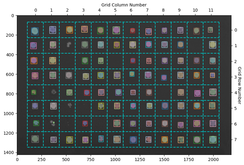
Here the objects with a colored overlay over them represent the different objects detected in your image. The boxes show the objects belonging to a specific grid section. The HeavyWatershedPipeline takes steps to ensure only one object in each section remains for downstream analysis. In reality, more objects were probably detected, but the refinement steps removed them according tos trict filters