6. Fitting Logistic Growth Curves

---

Background

In this tutorial we will cover how to fit growth curves on data from PhenoTypic. For growth curves you’ll typically want to use metrics of size from pht.measure.MeasureSize: “Size_Area” or “Size_IntegratedIntensity”. These can also be obtained from pht.measure.MeasureArea or pht.measure.MeasureIntensity respectively.

Size Metric Comparison:

Metric	Pros	Cons
“Shape_Area”	Simple to set up Captures lateral growth	Misses Vertical Growth
“Intensity_IntegratedIntensity”	Captures lateral and vertical growth	Requires color correction if there’s significant color drift or lots of color variation between colonies

Phenotypic uses the following form of the logistic formula:

Logistic Kinetics Model

\(N(t) = \frac{K } {1 + \frac{K - N0}{N0} e^{-r t}}\)

\(N_t\): population size at time t

\(N_0\): initial population size at time t

\(r\): growth rate

\(K\): Carrying capacity (maximum population size).

from which we can derive:

\(µ_{max} = \frac{Kr}{4}\)

\(µ_{max}\): maximum specific growth rate

To solver for the parameters, we use the following loss function with the scipy linear least squares solver

Loss Function

\(J(K,N_0,r) = \frac{1}{n}\sum_{i=1}^{n}\frac{1}{2}(f_{K,N0,r}(t^{(i)}) - N_t^{(i)})^2) + \lambda(\frac{dN}{dt}^2 + N_0^2) + \alpha \frac{\lvert K-\max({N_t})\rvert}{N_t}\)

\(\lambda\): regularization term for growth rate and initial population size

\(\alpha\): penalty term for deviations in the carrying capacity relative to the largest measurement

Overview

The data in this tutorial comes from the {doc} QuickStart tutorial

In this tutorial we use the following:

• pht.analysis.LogGrowthModel

• pht.analysis.TukeysOutlierRemover

• pht.analysis.EdgeCorrector

import phenotypic as pht

meas = pht.data.load_quickstart_meas()
meas.head()

Adding in metadata post-analysis for downstream processing

The original naming rule for this data was {Time}_{PlateSet}{Media}_{Replicate}

Based on this naming rule, let’s add the remaining metadata. These methods are all from pandas.DataFrame.

Note: This was the original naming rule, but it leads to some awkward splitting. It’s usually better to separate independent variables with underscores and related variables with dashes.

# We split the ImageName using string and then unpack that into three new columns in the dataframe
meas[["Metadata_Time", "Metadata_SetMedia", "Metadata_Replicate"]] = meas[
    "Metadata_ImageName"
].str.split("_", expand=True)

# Lets now split the {PlateSet}{Media} into different columns too
meas[["Metadata_PlateSet", "Metadata_Media"]] = meas["Metadata_SetMedia"].str.split(
    "", expand=True
)[[1, 2]]

# Time is a number, but because we split it from its name we need to convert it to the proper datatype
meas["Metadata_Time"] = meas["Metadata_Time"].astype(int)
meas["Metadata_PlateSet"] = meas["Metadata_PlateSet"].astype(int)

# Lets see our newest changes
meas[
    [
        "Metadata_ImageName",
        "Metadata_Time",
        "Metadata_PlateSet",
        "Metadata_Media",
        "Metadata_Replicate",
    ]
].head()

	Metadata_ImageName	Metadata_Time	Metadata_PlateSet	Metadata_Media	Metadata_Replicate
0	2_1S_5	2	1	S	5
1	2_1S_5	2	1	S	5
2	2_1S_5	2	1	S	5
3	2_1S_5	2	1	S	5
4	2_1S_5	2	1	S	5

Adding in metadata like strain name

While you can add the metadata per-image, its necessary to add it in post-extraction for things like colony strain names. To add in metadata like the strain name for each column to your data, we’ll use table joining.

# Lets generate a synthetic table of strain names
import pandas as pd

# It's important to use the same names as the measurement dataframe
synth_names = pd.DataFrame(
    data={
        "Metadata_PlateSet": 1,
        "Grid_SectionNum": range(96),
        "Metadata_StrainName": [f"SYNTH-{idx:02d}" for idx in range(96)],
    }
)

synth_names

	Metadata_PlateSet	Grid_SectionNum	Metadata_StrainName
0	1	0	SYNTH-00
1	1	1	SYNTH-01
2	1	2	SYNTH-02
3	1	3	SYNTH-03
4	1	4	SYNTH-04
...	...	...	...
91	1	91	SYNTH-91
92	1	92	SYNTH-92
93	1	93	SYNTH-93
94	1	94	SYNTH-94
95	1	95	SYNTH-95

96 rows × 3 columns

meas = meas.merge(synth_names, on=["Metadata_PlateSet", "Grid_SectionNum"], how="inner")
meas[
    ["Metadata_PlateSet", "Grid_SectionNum", "Metadata_StrainName", "Shape_Area"]
].head()

	Metadata_FileSuffix	Metadata_BitDepth	Metadata_ImageType	Metadata_ImageName	ObjectLabel	Bbox_CenterRR	Bbox_CenterCC	Bbox_MinRR	Bbox_MinCC	Bbox_MaxRR	...	ColorHSV_BrightnessStdDev	ColorHSV_BrightnessCoeffVar	ColorLab_ChromaEstimatedMean	ColorLab_ChromaEstimatedMedian	Metadata_Time	Metadata_SetMedia	Metadata_Replicate	Metadata_PlateSet	Metadata_Media	Metadata_StrainName
0	.jpg	8	GridImage	2_1S_5	1	143.066954	638.928742	116	616	171	...	0.020981	0.068122	2.324505	2.412023	2	1S	5	1	S	SYNTH-03
1	.jpg	8	GridImage	2_1S_5	2	150.888348	489.121803	122	464	182	...	0.049686	0.131528	2.861581	3.057672	2	1S	5	1	S	SYNTH-02
2	.jpg	8	GridImage	2_1S_5	3	152.518557	962.014356	122	934	185	...	0.046833	0.115846	3.028543	3.214427	2	1S	5	1	S	SYNTH-05
3	.jpg	8	GridImage	2_1S_5	4	152.439723	1610.904644	125	1589	182	...	0.045290	0.116357	4.114455	4.538226	2	1S	5	1	S	SYNTH-09
4	.jpg	8	GridImage	2_1S_5	5	156.673430	802.163285	129	779	185	...	0.043493	0.113999	2.941698	3.139710	2	1S	5	1	S	SYNTH-04

5 rows × 178 columns

# Lets isolate the measurements we care about
meas = meas[
    [
        "Metadata_ImageName",
        "Grid_SectionNum",
        "Metadata_Media",
        "Metadata_PlateSet",
        "Metadata_Replicate",
        "Metadata_StrainName",
        "Metadata_Time",
        "Shape_Area",
    ]
].sort_values(by=["Metadata_StrainName", "Metadata_Time"])

meas["Metadata_Time"] = meas["Metadata_Time"].astype(
    int
)  # Ensures that the time column is numeric
meas.head(10)

	Metadata_ImageName	Grid_SectionNum	Metadata_Media	Metadata_PlateSet	Metadata_Replicate	Metadata_StrainName	Metadata_Time	Shape_Area
8	2_1S_5	0	S	1	5	SYNTH-00	2	2295.0
89	2_1S_6	0	S	1	6	SYNTH-00	2	2420.0
171	2_1S_7	0	S	1	7	SYNTH-00	2	2751.0
315	3_1S_5	0	S	1	5	SYNTH-00	3	2676.0
401	3_1S_6	0	S	1	6	SYNTH-00	3	2877.0
485	3_1S_7	0	S	1	7	SYNTH-00	3	3206.0
568	3_1S_8	0	S	1	8	SYNTH-00	3	2840.0
651	4_1S_5	0	S	1	5	SYNTH-00	4	2948.0
740	4_1S_6	0	S	1	6	SYNTH-00	4	3413.0
826	4_1S_7	0	S	1	7	SYNTH-00	4	3535.0

Filtering and correction

In automated image processing, depending on the scene, objects can be:

• oversegmented (some of the background is detected along with the object)

• undersegmented (some of the object is not detected with the object)

• noise that was detected as an object

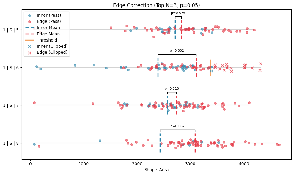
Other factors that may mess with our growth curves include stochastic biological noise or experimental error as well. To refine the data to reflect the true growth kinetics better, we can apply tukey’s outlier and our edge correction method on the dataset.

from phenotypic.analysis import TukeyOutlierRemover

tukey_outlier_analysis = TukeyOutlierRemover(
    on="Shape_Area", groupby=["Metadata_StrainName", "Metadata_Time"]
)

tukey_results = tukey_outlier_analysis.analyze(meas)

tukey_outlier_analysis.show(collapsed=True)

Warning: Displaying only first 20 of 451 groups

(<Figure size 1000x1200 with 1 Axes>,
 <Axes: xlabel='Shape_Area', ylabel='Group'>)

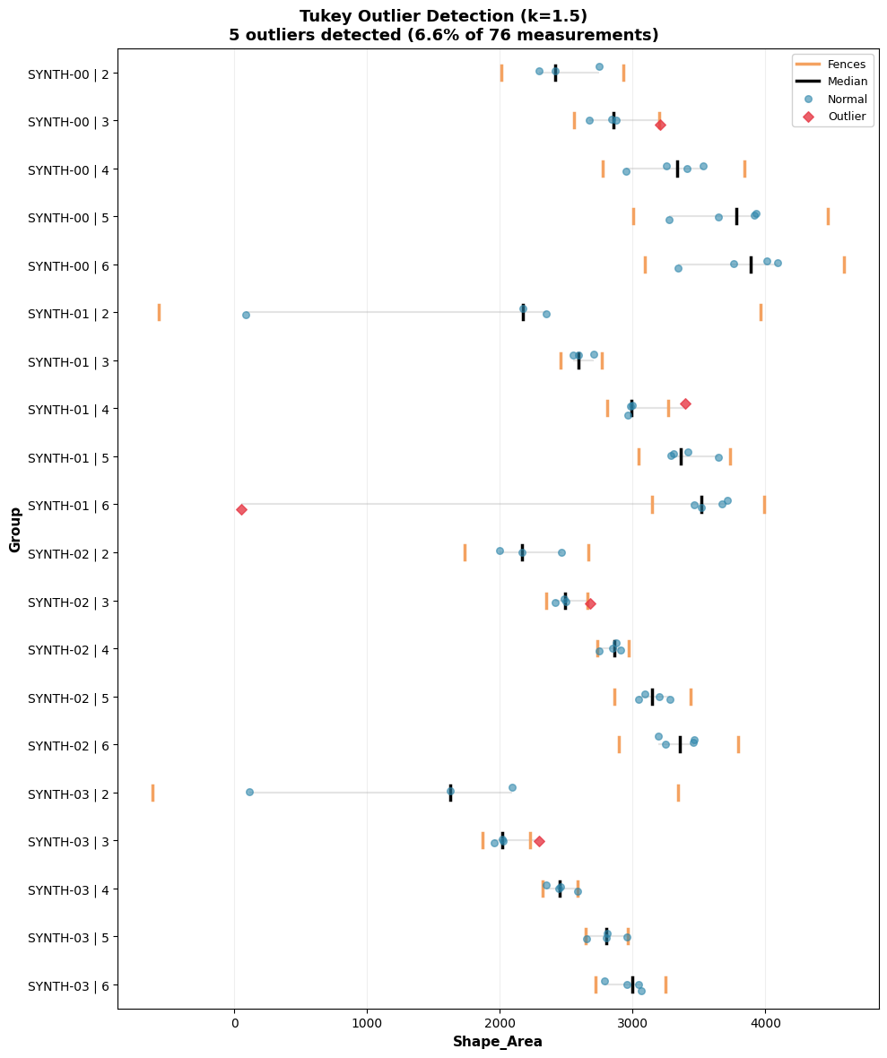
Since there’s a large amount of groups and they can’t all be displayed, only the first 20 are displayed, but this can be changed.

from phenotypic.analysis import EdgeCorrector

edge_correcter = EdgeCorrector(
    on="Shape_Area",
    groupby=["Metadata_PlateSet", "Metadata_Media", "Metadata_Replicate"],
    time_label="Metadata_Time",
)

edge_corrected = edge_correcter.analyze(tukey_results)
edge_correcter.show(collapsed=True)

(<Figure size 1000x600 with 1 Axes>,
 <Axes: title={'center': 'Edge Correction (Top N=3, p=0.05)'}, xlabel='Shape_Area'>)

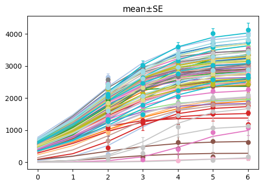
Fit model

New parameters: > lam: The regularization factor for specific growth rate > alpha: The penalty term for the relative deviation from the max of the carrying capacity

log_model = pht.analysis.LogGrowthModel(
    on="Shape_Area",
    groupby=["Metadata_StrainName"],
    agg_func="mean",
    time_label="Metadata_Time",
    lam=0.5,
    alpha=2.0,
    n_jobs=-1,
)
model_fit = log_model.analyze(meas)
model_fit.head()

	Metadata_StrainName	LogGrowthModel_r	LogGrowthModel_K	LogGrowthModel_N0	LogGrowthModel_µmax	LogGrowthModel_Kmax	LogGrowthModel_NumSamples	LogGrowthModel_OptimizerLoss	LogGrowthModel_OptimizerStatus	LogGrowthModel_MAE	LogGrowthModel_MSE	LogGrowthModel_RMSE
0	SYNTH-00	0.882962	3803.000000	731.050357	839.475765	3803.00	5	359014.371364	2	111.664757	19690.330182	140.322237
1	SYNTH-01	1.062408	3262.010706	363.235125	866.396198	3414.25	5	348964.083825	2	212.846392	51327.417300	226.555550
2	SYNTH-02	0.861747	3321.531212	663.466829	715.579876	3341.25	5	285067.340599	2	100.423547	18802.656973	137.122781
3	SYNTH-03	0.903318	2963.500000	347.147868	669.245998	2963.50	5	155206.330925	2	63.041344	5242.347575	72.404058
4	SYNTH-04	0.885146	3032.000000	593.850922	670.940923	3032.00	5	236673.126701	2	93.985535	14387.186777	119.946600

Parameters:

• on: What column to measure on

• groupby: What columns to form groups on. See also: pandas.DataFrame.groupby()

• agg_func: How to aggregate replicate time points. Default is “mean”. For other options see: pandas.DataFrame.agg()

• time_label: What column is to use for the time measurement. This should be added by the user either as metadata or externally.

Display results

log_model.show()

(<Figure size 600x400 with 1 Axes>, <Axes: title={'center': 'mean±SE'}>)

log_model.show(criteria={"Metadata_StrainName": ["SYNTH-00"]})

(<Figure size 600x400 with 1 Axes>, <Axes: title={'center': 'mean±SE'}>)

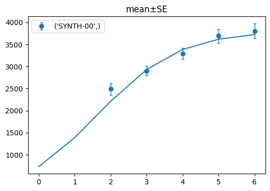
If we want to display only one of the strains, we can use the criteria like above. You can specify which column you want to filter by as a key and provide the