3. Understanding the Image Class: Data Components and Accessors#
This tutorial provides a comprehensive guide to the PhenoTypic Image class architecture, focusing on its main data components and how they interact with detection and analysis modules.
Learning Objectives#
By the end of this tutorial, you will understand:
The Image class hierarchy and accessor pattern
The six main data components:
rgb,gray,enh_gray,objmask,objmap, andmetadataHow these components interact during image processing workflows
When and how to use each component in your analysis
[1]:
# Import required libraries
import phenotypic as pht
import numpy as np
import matplotlib.pyplot as plt
Loading an Image and Basic Properties#
Let’s start by loading a sample plate image from the built-in dataset. We’ll use an image of bacterial colonies growing on agar media.
[2]:
# Load a sample plate image (12 hours of growth)
image = pht.data.load_colony(mode="Image")

# Display basic properties
print(f"Image name: {image.name}")
print(f"Image shape: {image.shape}")
print(f"Bit depth: {image.bit_depth}")
print(f"Data type: {type(image)}")
Image name: later_colony
Image shape: (200, 162, 3)
Bit depth: 8
Data type: <class 'phenotypic.core._image.Image'>
[3]:
# Visualize the original image
image.show()
[3]:
(<Figure size 800x600 with 1 Axes>, <Axes: >)
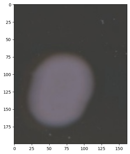
Image.show() will show the original input (either rgb or grayscale)
RGB Component: Multichannel Color Data#
The ``rgb`` accessor provides access to the multichannel RGB representation of the image.
Key Characteristics:#
Data type: uint8 (for 8-bit) or uint16 (for 16-bit images)
Shape:
(height, width, 3)- three channels for Red, Green, BlueAccess pattern: Use bracket notation
image.rgb[:]to get the arrayAutomatically set: When loading a color image
Empty for grayscale: If you load a 2D array, RGB remains empty
Related Operations:#
ImageCorrector: Can apply different types of corrections to this layerMeasureFeature: Color measurements are extracted from this component
[4]:
# Access the RGB data
rgb_data = image.rgb[:]

print(f"RGB shape: {rgb_data.shape}")
print(f"RGB dtype: {rgb_data.dtype}")
print(f"RGB value range: [{rgb_data.min()}, {rgb_data.max()}]")
print(f"\nIs RGB empty? {image.rgb.isempty()}")
RGB shape: (200, 162, 3)
RGB dtype: uint8
RGB value range: [55, 127]

Is RGB empty? False
[5]:
image.rgb.show()
[5]:
(<Figure size 800x600 with 1 Axes>, <Axes: >)

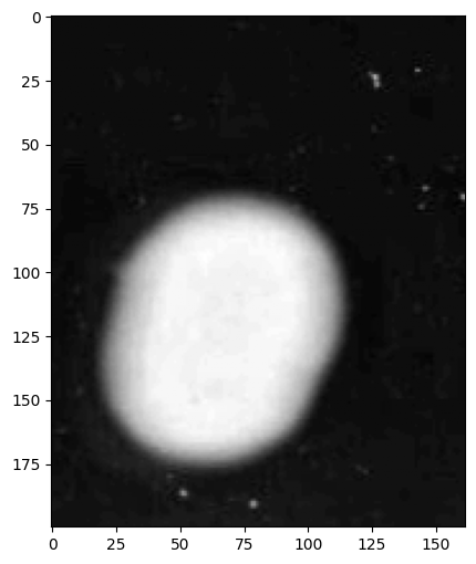
Gray Component: Grayscale Representation#
The ``gray`` accessor provides the grayscale representation of the image using weighted luminance conversion.
Key Characteristics:#
Data type: float32 with values in [0, 1] range
Shape:
(height, width)- single channelConversion: Automatically created from RGB using
skimage.color.rgb2grayWeighted formula:
0.2125*R + 0.7154*G + 0.0721*B(ITU-R BT.709)Read-only: Changes to gray won’t modify RGB (use
enh_grayfor modifications)Always present: Even for grayscale-loaded images
The grayscale information is also the intensity information. Certain corrections like flat-field operate on this layer, but don’t affect the RGB information. Thus, we keep it loaded in memory.
Related Operations:#
ImageCorrector’s: can apply different corrections to this componentMeasureFeature’s: measure different object features such as intensity from this layer
[6]:
# Access the grayscale data
gray_data = image.gray[:]

print(f"Gray shape: {image.gray.shape}")
print(f"Gray dtype: {image.gray.dtype}")
print(f"Gray value range: [{gray_data.min():.4f}, {gray_data.max():.4f}]")
print(f"\nIs gray empty? {image.gray.isempty()}")
Gray shape: (200, 162)
Gray dtype: float64
Gray value range: [0.2269, 0.4574]

Is gray empty? False
[7]:
# Visualize grayscale conversion
image.gray.show()
print(
    "\n💡 Note: The grayscale conversion preserves perceptual brightness better than simple averaging."
)
💡 Note: The grayscale conversion preserves perceptual brightness better than simple averaging.
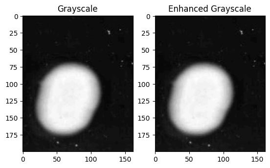
Enhanced Gray Component: Mutable Processing Copy#
The ``enh_gray`` accessor provides a mutable copy of the grayscale image for preprocessing, enhancement, and detection.
Key Characteristics:#
Data type: float32 with values in [0, 1] range
Shape:
(height, width)- single channelInitialization: Starts as an exact copy of
grayMutable: Can be modified without affecting the original
grayPrimary use: Detection algorithms process
enh_grayto create targets while, the original grayscale is preserved.Workflow: Apply enhancement operations → Detector uses
enh_gray→ Original stays intact
Many traditional computer vision operations operate on the grayscale matrix for calculations. Thus, Image.enh_gray.histogram() is a powerful tool for deciding what operations our images need to process. PhenoTypic uses a two-path strategy for measurement and detection. Many operations that improve object detection affect the data integrity of the original grayscale, which is used for intensity measurements. Thus, we incorporate the enh_gray matrix which is a copy of the original
grayscale matrix used for operations that enhance detection. Operations for enhancing detection can be found in phenotypic.enhace.
Related Operations:#
ImageEnhancer: Improves different aspects of the image such as contrast to this componentObjectDetector: Utilizes different algorithms to detect objects in this version of the image
[8]:
# Access enhanced grayscale data
enh_gray_data = image.enh_gray[:]

print(f"Enhanced gray shape: {enh_gray_data.shape}")
print(f"Enhanced gray dtype: {enh_gray_data.dtype}")
print(
    f"Enhanced gray value range: [{enh_gray_data.min():.4f}, {enh_gray_data.max():.4f}]"
)

# Check if enh_gray starts as a copy of gray
print(
    f"\nAre gray and enh_gray initially equal? {np.allclose(gray_data, enh_gray_data)}"
)
print(f"Are they the same object? {np.shares_memory(gray_data, enh_gray_data)}")
Enhanced gray shape: (200, 162)
Enhanced gray dtype: float64
Enhanced gray value range: [0.2269, 0.4574]

Are gray and enh_gray initially equal? True
Are they the same object? False
[9]:
fig, axes = plt.subplots(ncols=2)
image.gray.show(ax=axes[0], title="Grayscale")
image.enh_gray.show(ax=axes[1], title="Enhanced Grayscale")

print(
    "\n💡 Note: Enhancement operations can be applied to enh_gray without affecting the original gray data."
)
💡 Note: Enhancement operations can be applied to enh_gray without affecting the original gray data.
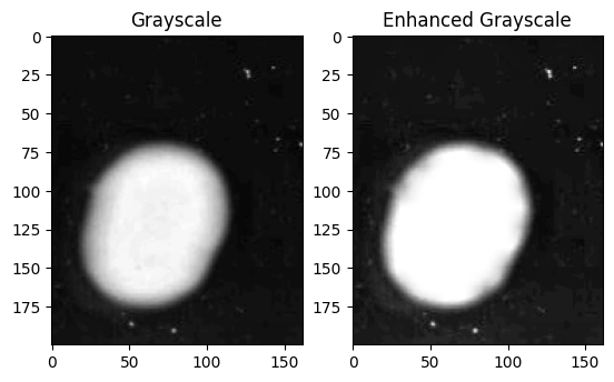
[10]:
pht.enhance.CLAHE().apply(image, inplace=True)

fig, axes = plt.subplots(ncols=2)
image.gray.show(ax=axes[0], title="Grayscale")
image.enh_gray.show(ax=axes[1], title="Enhanced Grayscale")

print(
    "\n💡 Note: Enhancement operations can be applied to enh_gray without affecting the original gray data."
)
💡 Note: Enhancement operations can be applied to enh_gray without affecting the original gray data.
Object Mask and Object Map: Detection Results#
The ``objmask`` and ``objmap`` accessors store the results of object detection algorithms. Let’s apply the OtsuDetector to see them in action.
OtsuDetector Workflow:#
Reads
enh_graydataCalculates optimal threshold using Otsu’s method
Creates binary mask and stores in
objmaskLabels connected regions and stores in
objmap
[11]:
# Apply OtsuDetector to detect colonies
detector = pht.detect.OtsuDetector(ignore_zeros=True, ignore_borders=True)
detector.apply(image, inplace=True)

print("✅ Detection complete!")
print(f"Number of detected objects: {image.num_objects}")
✅ Detection complete!
Number of detected objects: 6
6.1 Object Mask: Binary Representation#
The ``objmask`` is a binary mask showing which pixels belong to detected objects.
Key Characteristics:#
Values: 0 (background) and 1 (object pixels)
Shape:
(height, width)- matches image dimensionsStorage: Backed by sparse CSC matrix for memory efficiency
Mutable: Can be modified (triggers automatic objmap relabeling)
Set by: Detection algorithms (Otsu, Watershed, etc.)
[12]:
# Access object mask
objmask_data = image.objmask[:]

print(f"Object mask shape: {objmask_data.shape}")
print(f"Object mask dtype: {objmask_data.dtype}")
print(f"Unique values: {np.unique(objmask_data)}")
print(f"Number of object pixels: {np.sum(objmask_data)}")
print(f"Number of background pixels: {np.sum(objmask_data == 0)}")
print(
    f"Percentage of image covered by objects: {100 * np.sum(objmask_data) / objmask_data.size:.2f}%"
)
Object mask shape: (200, 162)
Object mask dtype: int64
Unique values: [0 1]
Number of object pixels: 7519
Number of background pixels: 24881
Percentage of image covered by objects: 23.21%
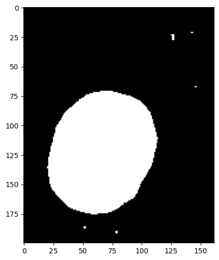
[13]:
# Visualize the object mask
image.objmask.show()

print(
    "\n💡 Note: The binary mask shows all detected object pixels without distinguishing individual objects."
)
💡 Note: The binary mask shows all detected object pixels without distinguishing individual objects.
6.2 Object Map: Labeled Regions#
The ``objmap`` assigns a unique integer ID to each connected region in the object mask.
Key Characteristics:#
Values: 0 (background) and unique integers for each object (1, 2, 3, …)
Shape:
(height, width)- matches image dimensionsStorage: Sparse CSC matrix (shared backend with objmask)
Automatic labeling: Created/updated when objmask changes
Used for: Individual object analysis, measurements, slicing
[14]:
# Access object map
objmap_data = image.objmap[:]

print(f"Object map shape: {objmap_data.shape}")
print(f"Object map dtype: {objmap_data.dtype}")
print(f"Number of unique objects: {len(np.unique(objmap_data)) - 1}")
print(f"Object IDs range: {objmap_data[objmap_data > 0].min()} to {objmap_data.max()}")
print(f"\nFirst 10 object IDs: {sorted(np.unique(objmap_data[objmap_data > 0]))[:10]}")
Object map shape: (200, 162)
Object map dtype: uint16
Number of unique objects: 6
Object IDs range: 1 to 6

First 10 object IDs: [np.uint16(1), np.uint16(2), np.uint16(3), np.uint16(4), np.uint16(5), np.uint16(6)]
[15]:
# Visualize the labeled object map
fig, axes = plt.subplots(1, 3, figsize=(16, 5))

# Object mask (binary)
axes[0].imshow(objmask_data, cmap="binary")
image.objmask.show(
    ax=axes[0], title=f"Object Mask\n(Binary: {image.num_objects} objects)"
)

# Object map (labeled)
image.objmap.show(
    ax=axes[1], title=f"Object Map\n(Binary: {image.num_objects} objects)"
)

# Overlay on original
axes[2].imshow(rgb_data)

image.show_overlay(ax=axes[2], title="Overlay")

plt.tight_layout()
plt.show()

print("\n💡 Note: Each color in the object map represents a distinct detected colony.")
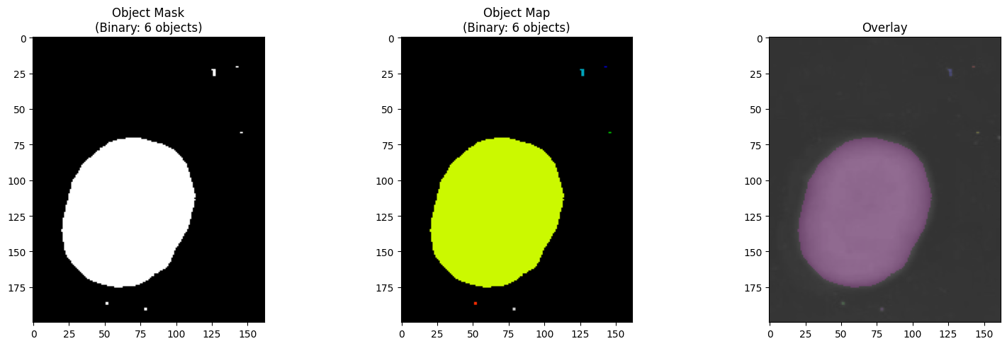
💡 Note: Each color in the object map represents a distinct detected colony.
Relationship Between objmask and objmap#
The objmask and objmap are tightly coupled:
Shared backend: Both use the same sparse CSC matrix storage
objmask → objmap: Binary mask shows “where objects are”
objmap → objmask: Labeled map shows “which object each pixel belongs to”
Automatic sync: Modifying objmask triggers relabeling of objmap
[16]:
# Demonstrate the relationship
print("Relationship verification:")
print(f"objmask non-zero pixels: {np.count_nonzero(objmask_data)}")
print(f"objmap non-zero pixels: {np.count_nonzero(objmap_data)}")
print(
    f"Are non-zero locations identical? {np.all((objmask_data > 0) == (objmap_data > 0))}"
)

print(f"\nobjmask values: {np.unique(objmask_data)}")
print(
    f"objmap values: {len(np.unique(objmap_data))} unique (0 + {image.num_objects} objects)"
)
Relationship verification:
objmask non-zero pixels: 7519
objmap non-zero pixels: 7519
Are non-zero locations identical? True

objmask values: [0 1]
objmap values: 7 unique (0 + 6 objects)
Metadata: Image Information Storage#
The ``metadata`` accessor provides a three-tier system for storing image information.
Three-Tier System:#
Private: Internal system use only
UUID for unique identification
Not directly modifiable by users
Protected: System-managed metadata
image_name: Image identifierbit_depth: 8 or 16 bitimage_type: BASE, OBJECT, or GRIDCan be read but modification is restricted
Public: User-modifiable metadata
Custom key-value pairs
Experimental conditions, timestamps, etc.
Fully modifiable by users
[17]:
# Access metadata
print("=" * 50)
print("METADATA CONTENTS")
print("=" * 50)

print("\n" + "-" * 50)
print("Key metadata values:")
print("-" * 50)
print(f"Name: {image.metadata['ImageName']}")
print(f"Bit depth: {image.metadata['BitDepth']}")
print(f"Image type: {image.metadata['ImageType']}")

image.metadata.table()
==================================================
METADATA CONTENTS
==================================================

--------------------------------------------------
Key metadata values:
--------------------------------------------------
Name: later_colony
Bit depth: 8
Image type: Image
[17]:
FileSuffix                                    .png
ImageName                             later_colony
ImageType                                    Image
BitDepth                                         8
UUID          635e302d-5501-4b9b-aa50-604281c8493a
Name: later_colony, dtype: object
[18]:
# Add custom metadata (public tier)
image.metadata["experiment_id"] = "EXP_001"
image.metadata["growth_time_hours"] = 12
image.metadata["strain"] = "Kluveromyces Marxianus"
image.metadata["temperature_celsius"] = 37.0
image.metadata["media_type"] = "LB Agar"

image.metadata.table()
[18]:
FileSuffix                                             .png
experiment_id                                       EXP_001
growth_time_hours                                        12
strain                               Kluveromyces Marxianus
temperature_celsius                                    37.0
media_type                                          LB Agar
ImageName                                      later_colony
ImageType                                             Image
BitDepth                                                  8
UUID                   635e302d-5501-4b9b-aa50-604281c8493a
Name: later_colony, dtype: object
Practical Tips and Best Practices#
When to Use Each Component#
Component |
Use When You Need To… |
|---|---|
rgb |
Access color information, display full-color images, analyze individual color channels |
gray |
Work with intensity data, maintain original data integrity, perform measurements |
enh_gray |
Apply preprocessing, test enhancement algorithms, prepare for detection |
objmask |
Work with binary masks, perform morphological operations, modify detection results |
objmap |
Analyze individual objects, measure per-object properties, extract specific colonies |
metadata |
Store experimental context, track processing parameters, organize datasets |
Accessor Pattern Benefits#
Consistent Interface: All accessors use bracket notation
[:]Data Integrity: Read-only accessors prevent accidental modifications
Automatic Sync: Changes to objmask automatically update objmap
Memory Efficiency: Sparse storage for object maps saves memory
Type Safety: Accessors enforce correct data types
Read-Only vs Mutable Components#
Read-Only (viewing via [:] returns non-writable views):
rgb: Preserve color data integritygray: Maintain original grayscale reference
Mutable (can be modified in-place):
enh_gray: Designed for preprocessingobjmask: Can be refined post-detectionobjmap: Automatically updates with objmaskmetadata: Fully modifiable for custom data
Integration with Other PhenoTypic Modules#
Detection (phenotypic.detect):
from phenotypic.detect import OtsuDetector, WatershedDetector
detector = OtsuDetector()
detector.apply(image)  # Populates objmask and objmap
Enhancement (phenotypic.enhance):
from phenotypic.enhance import CLAHE, GaussianBlur
enhancer = CLAHE()
enhancer.apply(image)  # Modifies enh_gray
Refine (phenotypic.refine):
from phenotypic.refine import BorderObjectRemover
refiner = BorderObjectRemover()
results = refiner.apply(image)  # uses objmask and objmap and cleans the detection results
Measurement (phenotypic.measure):
from phenotypic.measure import MeasureSize
measurer = MeasureSize()
results = measurer.apply(image)  # Uses objmap for per-object analysis
Analysis (phenotypic.analysis):
# Access individual objects using objmap labels
for obj in image.objects:
    print(f"Object {obj.label}: Area = {obj.area}")
[ ]: