Tutorial 1: Your First Plate Image

Welcome to PhenoTypic! In this tutorial, you will load your first agar plate image, understand the difference between the base Image and the grid-aware GridImage classes, and explore the accessor pattern that gives you different views of the same image.

Most arrayed colony workflows use GridImage, but understanding that it builds on the same Image interface will make the rest of the tutorials feel much more natural.

By the end of this tutorial you will know how to:

1. Load a plate image as either an Image or a GridImage

2. Understand when to use each class

3. Inspect basic properties: .shape, .bit_depth, .name, and .dtype

4. Explore the three key image layers using .show()

5. Display a plate interactively with .dash()

Imports

Let’s start with the standard PhenoTypic import. The convention throughout these tutorials is import phenotypic as pht.

import phenotypic as pht
from phenotypic.data import load_yeast_plate

Load a Plate Image

PhenoTypic ships with sample plate images so you can start experimenting straight away. load_yeast_plate() returns a GridImage by default — a 2-by-4 crop of an arrayed Rhodotorula yeast plate.

You can also wrap the same pixel data in a plain Image. Here’s the difference in one sentence: use Image when the plate doesn’t have a meaningful row-and-column layout; use GridImage when well position matters (which is almost always the case for arrayed phenotyping).

plate_array = load_yeast_plate(mode="array")
image = pht.Image(plate_array, name="yeast_plate_image")
plate = load_yeast_plate()

print(f"Base image:                {type(image).__name__}")
print(f"Grid plate:                {type(plate).__name__}")
print(f"GridImage is also an Image: {isinstance(plate, pht.Image)}")

Base image:                Image
Grid plate:                GridImage
GridImage is also an Image: True

You now have two objects. image is a plain Image with pixel data, metadata, accessors, and visualization methods. plate is a GridImage — it has everything image has, plus a .grid accessor for row-and-column plate layout.

The rest of this tutorial uses plate because most PhenoTypic examples work with arrayed plates. Everything shown below also applies to a plain Image unless it explicitly uses .grid.

Inspect the Grid Layout

A GridImage knows the intended plate layout before detection. That becomes more useful once colonies are detected and each one can be assigned to a specific well. For now, let’s just confirm the plate format looks right.

print("Grid rows:    ", plate.grid.nrows)
print("Grid columns: ", plate.grid.ncols)
print("Grid sections:", plate.grid.nrows * plate.grid.ncols)

Grid rows:     2
Grid columns:  4
Grid sections: 8

Inspect Basic Properties

Before processing any plate it’s worth taking a moment to understand what you’re working with. A few key properties tell you almost everything you need to know.

Property	What it tells you
.shape	Image dimensions — (height, width, channels)
.bit_depth	Pixel precision — 8-bit means values 0–255; 16-bit means 0–65 535
.name	A human-readable identifier for this image
.rgb.dtype	The NumPy data type of the underlying pixel array

print("Shape:    ", plate.shape)
print("Bit depth:", plate.bit_depth)
print("Name:     ", plate.name)
print("Dtype:    ", plate.rgb.dtype)

Shape:     (770, 1644, 3)
Bit depth: 8
Name:      RhodotorulaYeastCenterCrop
Dtype:     uint8

The shape confirms this is a 3-channel (RGB) image. The bit depth and dtype tell you the precision of each pixel — important context before choosing enhancement or detection settings.

Exploring the Image Layers with .show()

PhenoTypic uses an accessor pattern to give you different representations of the same plate without making extra copies. Instead of calling separate functions, you read views through dot-notation attributes.

The three primary layers are:

Accessor	What it provides	Typical use
.rgb	Full-color pixel data	Visualization, color analysis
.gray	Luminance-weighted grayscale	Intensity-based measurements
.detect_mat	Detection matrix (enhanced grayscale)	Colony detection and segmentation

Each accessor has a .show() method that renders it as a static matplotlib figure. This is a great way to get a clear, side-by-side look at each layer as you learn what they are.

The RGB Layer

The .rgb accessor holds the original full-color image. You can use [:] to get the underlying NumPy array (shape: height × width × 3), or .show() to visualize it immediately. This is the starting point for all color analysis.

rgb_array = plate.rgb[:]
print("Shape:", rgb_array.shape)
print("Dtype:", rgb_array.dtype)

Shape: (770, 1644, 3)
Dtype: uint8

fig, ax = plate.rgb.show(title="RGB — full-color plate")

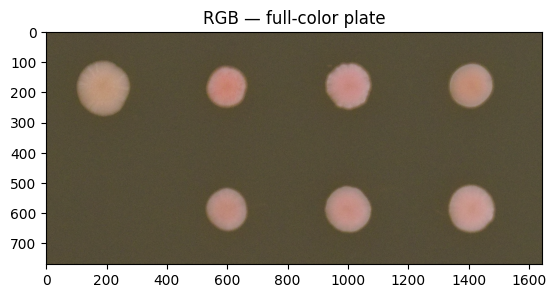
Take a look at those pigmented Rhodotorula colonies — bright, round spots on a light agar background. That color information is preserved untouched throughout the entire processing pipeline.

The Grayscale Layer

The .gray accessor provides a luminance-weighted grayscale version of the plate. The conversion uses perceptual weights so bright colonies appear bright and dark agar appears dark — matching what your eye expects.

The resulting array has shape (height, width) — a single channel — with float32 values.

gray_array = plate.gray[:]
print("Shape:", gray_array.shape)
print("Dtype:", gray_array.dtype)

Shape: (770, 1644)
Dtype: float32

fig, ax = plate.gray.show(title="Grayscale — luminance-weighted")

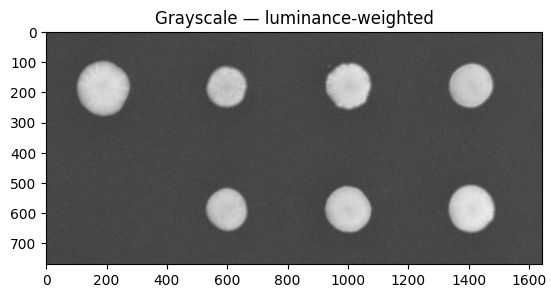
The Detection Matrix

The .detect_mat accessor is the layer that PhenoTypic’s detectors actually work on. When you apply enhancers to a plate, they modify this detection matrix while leaving .rgb and .gray untouched.

This is a deliberate design choice: you can aggressively preprocess .detect_mat to help detectors find colonies without corrupting the original color data you need for accurate measurements later.

Right now, before any enhancers have been applied, the detection matrix looks identical to the grayscale layer — that’s expected.

detect_array = plate.detect_mat[:]
print("Shape:", detect_array.shape)
print("Dtype:", detect_array.dtype)

Shape: (770, 1644)
Dtype: float32

fig, ax = plate.detect_mat.show(title="Detection matrix — ready for enhancers")

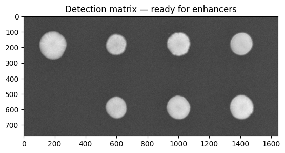
Right now .detect_mat looks just like .gray — and that’s exactly right. Once you start applying enhancers (contrast stretching, background subtraction, and so on), the detection matrix will diverge from the raw grayscale, making it much easier for detectors to find and segment colonies.

Interactive Display with .dash()

While .show() gives you clean static figures for exploring layers, PhenoTypic also provides .dash() for interactive Plotly visualizations. This is the preferred display method in tutorials and notebooks because you can zoom, pan, and hover to inspect pixel values.

Every accessor supports .dash() and the top-level .dash() on the image object itself delegates to .rgb by default.

# Full-color plate — interactive, zoomable
plate.dash()

# Detection matrix — useful for checking enhancer effects later
plate.detect_mat.dash()

Try zooming in on one of the colonies. The interactive viewer will be your best friend for diagnosing detection issues in later tutorials.

Summary

Great work — you have loaded your first plate image, compared Image and GridImage, inspected the image properties, and seen all three key image representations that PhenoTypic provides:

Concept	What you learned
Image	Base class for pixel data, metadata, accessors, and visualization
GridImage	Extends Image with .grid layout for arrayed plates
.rgb	Full-color data — preserved untouched through the pipeline
.gray	Perceptual grayscale for intensity-based work
.detect_mat	The detection matrix enhancers modify and detectors consume
.show()	Static matplotlib display — great for inspecting individual layers
.dash()	Interactive Plotly display — preferred for tutorial exploration

You now have a solid foundation for working with plate images in PhenoTypic.

Next up: In Tutorial 2: Detecting Colonies, you will use this plate to detect and segment individual colonies for the first time.